What This Post Covers
In our post on speculative decoding, we covered how a small draft model proposes tokens that a large target model verifies in parallel, achieving 2-3x speedups without changing the output distribution. That technique exploits idle GPU compute during memory-bound inference.
This post examines a follow-up question: can we make speculative decoding itself faster? The answer is yes. A recent paper by Kumar, Dao, and May (ICLR 2026) identifies a sequential bottleneck within standard speculative decoding and eliminates it through a technique called Speculative Speculative Decoding (SSD). Their algorithm, Saguaro, achieves up to 5x speedup over autoregressive decoding and roughly 2x over optimized speculative decoding.
We will walk through the bottleneck SSD targets, the core idea of speculating about verification outcomes, and the three engineering challenges that Saguaro solves: cache construction, cache-aware sampling, and batch-size scaling. Each section explains why the naive approach fails before presenting the solution.
The Hidden Bottleneck in Speculative Decoding
Standard speculative decoding runs in a loop: the draft model generates K tokens, the target model verifies them in a single forward pass, and the process repeats. This is faster than autoregressive decoding because verification amortizes the expensive memory read of the target model’s weights across multiple tokens.
But there is a sequential dependency hiding in plain sight. Let’s trace what happens on the draft model’s GPU during one round:
- The draft model generates K tokens (draft phase)
- The draft model sends tokens to the target model
- The target model runs verification (the draft model sits completely idle)
- The target model returns the verification outcome
- The draft model generates K new tokens for the next round
- Go to step 2
The draft model does nothing during step 3. If verification takes $T_v$ time units, the draft model wastes $T_v$ time units every round. Since the target model is much larger than the draft, $T_v$ dominates the round duration. The draft model’s GPU is idle for the majority of each round.
This is the bottleneck SSD eliminates. Instead of waiting for verification to finish, the draft model spends that idle time doing something useful: predicting what the verification outcome will be and pre-computing the next round’s speculation for each likely outcome.
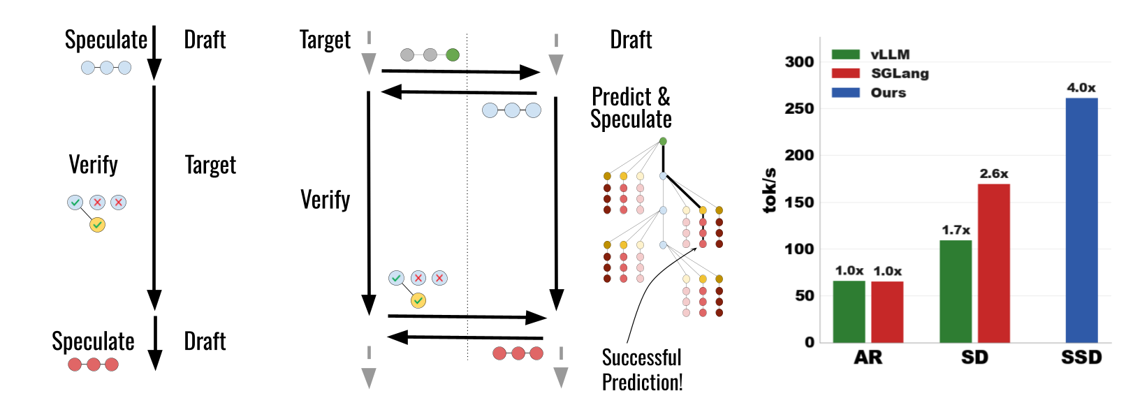
The Core Idea: Speculate About the Speculation
The idea draws from CPU speculative execution. When a CPU encounters a conditional branch, it does not wait for the condition to resolve. Instead, it predicts the likely outcome and begins executing instructions along that predicted path. If the prediction was correct, the results are kept. If wrong, they are discarded and the correct path is executed.
SSD applies this same principle to speculative decoding. While the target model verifies round $T$’s draft tokens, the draft model:
- Predicts what the verification outcome will be
- Pre-computes speculations for each likely outcome
- Stores these in a speculation cache
When verification finishes, the actual outcome is compared against the cache. If it matches a cached prediction (a cache hit), the next round’s speculation is returned instantly with zero drafting latency. If it doesn’t match (a cache miss), the system falls back to standard synchronous drafting.
What Is a Verification Outcome?
To understand what we need to predict, let’s define the verification outcome precisely. When the target model verifies K draft tokens, two things are determined:
- $k$: the number of accepted draft tokens (ranging from 0 to K)
- $t^*$: the bonus token, sampled from the target distribution at the first disagreement point (or at position K+1 if all tokens are accepted)
The verification outcome is the pair $v^T = (k, t^*)$. This fully determines the context from which the next round’s speculation must begin. If we can predict $v^T$ before verification completes, we can pre-compute the next K draft tokens starting from that context.
The Speculation Cache
The speculation cache $S^T$ is a dictionary that maps predicted verification outcomes to pre-computed speculations:
$$S^T : (k, t^*) \to (s_1, s_2, \ldots, s_K)$$Each entry contains K draft tokens generated autoregressively by the draft model starting from the context implied by $(k, t^*)$.
When verification returns the actual outcome $v^T$:
- Cache hit ($v^T \in S^T$): Return the cached speculation immediately. Zero drafting latency for this round.
- Cache miss ($v^T \notin S^T$): Fall back to generating a fresh speculation synchronously.
The Speculation Cache
Mapping predicted verification outcomes to pre-computed speculations
The key question is obvious: how do we choose which outcomes to cache? The space of possible outcomes is $(K+1) \times |V|$ where $|V|$ is the vocabulary size (typically 32,000-128,000). We cannot pre-compute speculations for all of them. This is the first of three challenges Saguaro addresses.
The Speedup Formula
Before diving into the three challenges, let’s quantify the potential. The expected speedup of SSD over autoregressive decoding (Theorem 7 from the paper) is:
$$\text{speedup}_{\text{SSD}} = \frac{p_{\text{hit}} \cdot E_{\text{hit}} + (1 - p_{\text{hit}}) \cdot E_{\text{miss}}}{p_{\text{hit}} \cdot \max(1, T_p) + (1 - p_{\text{hit}}) \cdot (1 + T_b)}$$Walking through each term: $p_{\text{hit}}$ is the probability of a cache hit. $E_{\text{hit}}$ and $E_{\text{miss}}$ are the expected number of tokens generated per round on a hit and miss respectively. $T_p$ is the latency of the primary speculator (the neural draft model) relative to the verifier, and $T_b$ is the latency of the backup speculator used on cache misses.
The numerator is the expected tokens per round, weighted by hit/miss probabilities. The denominator is the expected wall-clock time per round.
Two corollaries follow directly:
Corollary 8: SSD strictly outperforms standard speculative decoding whenever $p_{\text{hit}} > 0$. Any nonzero cache hit rate improves performance because cache hits eliminate drafting latency entirely, and cache misses simply revert to standard SD behavior.
Corollary 9: The maximum speedup is bounded by $(1 + T_{\text{SD}}) \cdot (E_{\text{hit}} / E_{\text{SD}})$, where $T_{\text{SD}}$ and $E_{\text{SD}}$ are the drafting time and expected tokens for standard SD. When the cache hit rate approaches 1, all drafting latency vanishes and we gain a factor of $(1 + T_{\text{SD}})$ in the denominator.
Challenge 1: Building the Cache (Saguaro Cache Construction)
The Problem
A verification outcome is a pair $(k, t^*)$. The acceptance length $k$ ranges from 0 to K (typically K=7 in SSD), giving K+1 possibilities. The bonus token $t^*$ comes from a vocabulary of size $|V|$. The total outcome space is $(K+1) \times |V|$, which is roughly 250,000 for K=7 and $|V|$=32,000.
We have a budget of $B$ speculations we can pre-compute during the verification window. Each speculation requires the draft model to run K autoregressive steps. With the verification latency of a 70B target model on 4 H100s, we can fit roughly $B = 20\text{-}30$ speculations. We need to choose wisely.
Decomposing the Problem
Saguaro decomposes this into two subproblems:
- For each acceptance length $k$, how many bonus tokens should we cache? Call this the fan-out $F_k$.
- For a given fan-out $F_k$, which bonus tokens should we cache?
The second question has a straightforward answer: use the top-$F_k$ tokens from the draft model’s own probability distribution at that position. The draft model has already computed logits during the current round’s speculation, so the most likely tokens are immediately available. Empirically, this predicts the actual bonus token with up to 90% accuracy at moderate fan-out.
The first question, how to allocate fan-out across positions, is where the interesting optimization happens.
What Is Fan-Out?
Each row is one possible acceptance length. Fan-out = how many bonus tokens we cache for that outcome.
Each purple cell is one pre-computed speculation (K draft tokens). The total number of cells = budget B.
Position k=K (all accepted) is boosted because the target distribution is sharper, making prediction easier.
Power-Law Cache Hits
The authors make a key empirical observation: cache miss probability follows a power law in the fan-out:
$$1 - p_{\text{hit}}(F) = \frac{1}{F^r}$$for some exponent $r > 0$ that depends on the draft-target alignment. This means that doubling the fan-out does not halve the miss rate. Instead, miss rate decreases polynomially, with diminishing returns as fan-out grows. This finding (confirmed across multiple model pairs and datasets) drives the allocation strategy.
Geometric Fan-Out
Given the power-law structure and a total budget $\sum_{k=0}^{K} F_k \leq B$, Saguaro solves a constrained optimization problem using Lagrange multipliers. The result (Theorem 12) is a geometric allocation:
$$F_k = F_0 \cdot \alpha_p^{k/(1+r)} \quad \text{for } k < K$$where $\alpha_p$ is the per-token acceptance rate and $F_0$ is determined by the budget constraint. The formula allocates more fan-out to earlier positions (small $k$) and less to later positions.
The reasoning: position $k=0$ (first token rejected) is more probable than $k=5$ (five tokens accepted before rejection) because each acceptance is an independent event with probability $\alpha_p < 1$. The probability of reaching acceptance length $k$ is roughly $\alpha_p^k \cdot (1 - \alpha_p)$, a geometric distribution. Allocating fan-out proportionally to the probability of each outcome maximizes the expected cache hit rate.
There is one exception: position $k=K$ (all tokens accepted) receives a boost. When all K draft tokens are accepted, the bonus token comes directly from the target model’s distribution $p_{\text{target}}$ rather than the residual distribution. The target distribution is sharper and more concentrated, making the top-$F$ prediction more accurate. Saguaro accounts for this with a multiplicative correction:
$$F_K = F_0 \cdot \alpha_p^{K/(1+r)} \cdot (1 - \alpha_p)^{-1/(1+r)}$$Geometric Fan-Out Allocation
How Saguaro distributes its speculation budget across acceptance positions
Why geometric works
The probability of reaching acceptance length k is roughly αk(1-α). Earlier positions are more likely, so they deserve more fan-out. Position K (all accepted) gets boosted because the bonus token comes from the sharper target distribution, making it easier to predict.
Challenge 2: Trading Acceptance for Cache Hits (Saguaro Sampling)
The Tension
There is a fundamental tension between two objectives in SSD. On one hand, we want the draft model to closely match the target model so that acceptance rates stay high. On the other hand, we want to predict the bonus token $t^*$ accurately so that cache hit rates stay high.
These objectives conflict. Here is why.
Recall from our speculative decoding post that the bonus token is sampled from the residual distribution:
$$r(\cdot) \propto \max(p_{\text{target}}(\cdot) - p_{\text{draft}}(\cdot), 0)$$When the draft model closely matches the target ($p_{\text{draft}} \approx p_{\text{target}}$), the acceptance rate is high but the residual $\max(p_{\text{target}} - p_{\text{draft}}, 0)$ is spread thinly across many tokens. A thin residual means the bonus token could be almost anything, making it hard to predict and reducing cache hit rates.
When the draft model diverges from the target, the residual concentrates on tokens where $p_{\text{target}} \gg p_{\text{draft}}$, making the bonus token more predictable. But acceptance rates drop, meaning fewer tokens per round.
The Solution: Intentional Misalignment
Saguaro sampling resolves this tension by deliberately modifying the draft model’s sampling distribution. For a set of cached tokens (the top-$F$ tokens at each position), Saguaro suppresses the draft model’s probability on those specific tokens:
$$\sigma_{F,C}(z) \propto \begin{cases} C \cdot \exp(z_t) & \text{if } t \in \text{top}_F(z) \\ \exp(z_t) & \text{otherwise} \end{cases}$$Here $z$ is the vector of draft model logits, $F$ is the fan-out, and $C \in [0,1]$ is a downweighting constant. When $C=1$, this is the standard softmax with no modification. When $C < 1$, the cached tokens receive reduced probability in the draft’s distribution.
Why does this help? Let’s trace the effect on the residual.
When the draft model assigns less probability to a cached token, the gap $p_{\text{target}}(\cdot) - p_{\text{draft}}(\cdot)$ becomes larger for that token. A larger gap means the residual distribution assigns more probability to that token. Saguaro is steering the entire residual distribution to concentrate on the exact tokens it has cached.
Saguaro Sampling: Trading Acceptance for Cache Hits
How downweighting cached tokens in the draft forces the residual to concentrate on those same tokens
Draft Distribution q(x) with Saguaro
Residual Distribution max(p - q, 0)
The tradeoff
Slide C toward 0 to see how suppressing draft probability on cached tokens (marked with purple dots) forces the residual distribution to concentrate on those same tokens. This increases cache hit rate at the cost of acceptance rate. The optimal C* balances both effects for maximum end-to-end speedup.
Theorem 15 from the paper confirms this formally: the cache hit rate $p_{\text{hit}}$ increases monotonically as $C \to 0$. Push $C$ all the way to zero and the residual distribution is forced entirely onto cached tokens (guaranteeing a hit), but the acceptance rate collapses because the draft distribution diverges maximally from the target.
The optimal $C^*$ balances these competing effects and depends on the sampling temperature:
- Temperature 0 (greedy decoding): $C = 1$ is optimal. The bonus token is deterministic (the argmax of the target distribution), so the top-1 draft prediction already has high accuracy. No need to sacrifice acceptance rate.
- High temperature: $C \ll 1$ becomes advantageous. The bonus token is sampled from a flatter distribution, making it harder to predict without help. Saguaro sampling concentrates the residual, recovering cache hit rates that would otherwise be low.
In practice, Saguaro sampling provides up to 50% additional end-to-end speedup at high temperatures compared to using $C=1$.
Challenge 3: Scaling to Large Batches (Saguaro Fallback)
The Batch Size Problem
Everything so far has assumed batch size 1 (a single sequence). At larger batch sizes, a new problem emerges.
With batch size $b$, the system can only proceed to the next round when all $b$ sequences have speculations ready. The probability that every sequence in the batch gets a cache hit is:
$$P(\text{all hit}) = p_{\text{hit}}^b$$Even with $p_{\text{hit}} = 0.9$ per sequence, a batch of 16 sequences gives $P(\text{all hit}) = 0.9^{16} \approx 0.19$. At batch size 32, it drops to $0.9^{32} \approx 0.03$. The probability of at least one cache miss grows exponentially, and a single miss stalls the entire batch.
The Naive Fallback Fails
The intuitive solution is simple: when a cache miss occurs, have the primary draft model generate a fresh speculation on the spot. But this is catastrophically bad at scale.
The primary draft model is still a neural network that generates tokens autoregressively. Generating K tokens takes non-trivial time. While this one stalled sequence catches up, every other sequence in the batch (including those with cache hits) waits. The batch is only as fast as its slowest member.
Corollary 16 in the paper formalizes this: at large batch sizes, the SSD speedup becomes overwhelmingly bounded by the fallback latency. If the fallback speculator is slow, the theoretical gains from caching vanish.
Dual-Tier Fallback
Saguaro solves this with a dual-tier fallback strategy controlled by a critical batch size $b^*$:
Below $b^*$ (low batch regime): Cache misses are infrequent. The primary draft model serves as its own fallback, generating a fresh speculation synchronously. The latency penalty is acceptable because misses are rare and each one affects only one sequence.
Above $b^*$ (high batch regime): The system switches to an ultra-fast backup speculator with minimal latency. This could be an n-gram model, random tokens, or a token frequency model. The backup’s speculations will likely be rejected during verification (random tokens have near-zero acceptance rate). But the strategic insight is that the latency cost of feeding bad speculations to one sequence is vastly less than the latency cost of making the entire batch wait for a neural draft model.
Theorem 17 proves this formally: accepting a single sequence’s quality penalty (poor speculation) is strictly better than inflicting the primary drafter’s latency across the entire batch.
The critical batch size $b^*$ is derived analytically from the speedup equation and depends on $p_{\text{hit}}$, $T_p$ (primary drafter latency), and $T_b$ (backup latency).
Dual-Tier Fallback Strategy
How batch size determines the optimal fallback speculator
Misses are infrequent. Quality matters more than speed.
Primary Draft (Neural)Misses are near-certain. Speed matters more than quality.
Fast Backup (n-gram/random)Why fast beats accurate at scale
At batch size 32 with 85% per-sequence hit rate, P(at least one miss) = 99.6%. A miss is nearly guaranteed every round. Using the primary neural draft as fallback would stall the entire batch for its generation time. A fast backup (even random tokens) unblocks the batch instantly, and only the single stalled sequence pays a quality penalty.
The Full Algorithm
SSD runs three concurrent processes: a main coordinator, a verifier, and a speculator. Here is the algorithm:
# Main: launches speculator asynchronously, runs verifier
def main(prompt, target, primary_draft, backup_draft):
    launch_async(speculator, prompt, primary_draft, backup_draft)
    return verifier(prompt, target)

# Verifier: runs on target model's GPUs (e.g., 4x H100)
def verifier(prompt, target):
    target.prefill(prompt)
    spec_tokens = RECEIVE()              # wait for first speculation
    generated = []

    while True:
        outcome = target.verify(spec_tokens)   # standard SD verification
        generated.extend(outcome.tokens)

        if EOS in outcome.tokens:
            return generated

        SEND(outcome)                          # send (k, t*) to speculator
        spec_tokens = RECEIVE()                # wait for next speculation

# Speculator: runs on draft model's GPU (e.g., 1x H100)
def speculator(prompt, primary_draft, backup_draft):
    primary_draft.prefill(prompt)
    spec_tokens = primary_draft.speculate(prompt)  # initial speculation

    while True:
        SEND(spec_tokens)                      # send to verifier

        # While verification runs, build the cache
        cache = build_speculation_cache(
            spec_tokens, primary_draft           # §4.1: geometric fan-out
        )

        outcome = RECEIVE()                     # get actual (k, t*)

        if EOS in outcome:
            return

        if outcome in cache:                    # CACHE HIT
            spec_tokens = cache[outcome]        # instant return
        else:                                   # CACHE MISS
            spec_tokens = fallback(             # §4.3: dual-tier
                outcome, primary_draft, backup_draft
            )
Step-by-Step: One Round
Let’s trace through a single round to see how the pieces fit together.
Step 1: The speculator sends K draft tokens to the verifier and immediately begins predicting outcomes. It examines the draft model’s logits at each position to determine the most likely bonus tokens.
Step 2: Using geometric fan-out (Challenge 1), the speculator allocates its budget across positions. For each predicted outcome $(k, t^*)$, it generates K new draft tokens autoregressively from that context.
Step 3: These speculations are stored in the cache. With K=7 and fan-out F=3, the cache contains roughly 24 entries (8 acceptance lengths, with 3 bonus token predictions each, weighted by geometric allocation).
Step 4: The verifier finishes and sends back the actual outcome $(k, t^*)$.
Step 5: Cache lookup. If the outcome matches, the cached speculation is returned instantly. If not, the fallback mechanism kicks in.
The critical property is that on a cache hit, the round latency equals only the verification time (because the speculation was pre-computed in parallel). In standard SD, the round latency equals verification time plus drafting time. This is where the speedup comes from.
Correctness: SSD Is Lossless
An important guarantee: SSD produces the same output distribution as standard speculative decoding (which itself matches autoregressive decoding exactly).
On a cache hit, the cached speculation is verified using the same rejection sampling mechanism as standard SD. The fact that the speculation was pre-computed rather than computed just-in-time changes nothing about verification correctness.
On a cache miss, the system falls back to standard synchronous SD, which is known to be lossless.
The speculation cache is a performance optimization that never affects what tokens the target model accepts or rejects. Pre-speculation only changes when the draft tokens are computed, not what they are or how they are verified.
Hardware Setup
SSD requires the draft and target models to run on separate GPUs so they can operate concurrently. The typical configuration:
- Target model (verifier): 4x H100 80GB GPUs with tensor parallelism (for Llama-3.1-70B)
- Draft model (speculator): 1x H100 80GB GPU on a separate device
- Total: 5 GPUs for SSD vs. 4 GPUs for standard SD/AR
This is a 25% increase in hardware. The question is whether the speedup justifies the extra cost. At batch size 1, SSD achieves roughly 2x higher throughput than SD with the same target model, meaning the throughput per GPU still improves substantially.
Results
The authors benchmark SSD (with Saguaro optimizations) against autoregressive decoding and standard speculative decoding across four datasets: HumanEval (code), Alpaca (chat), GSM8K (math), and UltraFeedback (general).
Setup: Llama-3.1-70B-Instruct as the target model on 4x H100 GPUs, Llama-3.2-1B-Instruct as the draft model on 1x H100 GPU. K=6 for SD, K=7 for SSD, fan-out F=3 for SSD.
Performance: AR vs SD vs SSD
Throughput comparison at batch size 1, greedy decoding (temperature = 0)
Target: 4x H100 80GB (TP=4) | Draft: 1x H100 80GB | K=6 (SD), K=7 (SSD), F=3
Key findings:
- SSD vs. autoregressive: Up to ~5x faster (e.g., 255.8 tok/s vs. 54.7 tok/s on some benchmarks)
- SSD vs. standard SD: Up to ~2x faster (255.8 vs. 161.8 tok/s)
- At larger batch sizes: SSD still provides ~20% improvement over SD, even as cache hit rates drop. The Saguaro optimizations push the throughput-latency Pareto frontier across all batch sizes.
- Temperature sensitivity: Cache hit rates decrease with sampling temperature, but Saguaro sampling (low $C$) compensates effectively, maintaining gains at high temperatures.
The results also confirm on Qwen-3-32B (target) with Qwen-3-0.6B (draft): 203.8 tok/s for SSD vs. 136.8 for SD vs. 88.8 for AR.
Where SSD Fits in the Landscape
SSD is not the first attempt to overlap drafting and verification. Several concurrent methods target the same bottleneck:
| Method | Approach | Limitation |
|---|---|---|
| AMUSD | Pre-speculates for the “all accepted” outcome only | Misses all partial-acceptance cases |
| PEARL | Single outcome prediction | Same limitation as AMUSD |
| SwiftSpec | Token tree branching off current speculation | Greedy only; fallback struggles at high temp/batch |
| SpecBranch | Single branching point with regular fallback | Approximately a special case of SSD |
| SSD (Saguaro) | Multi-outcome caching with geometric fan-out, cache-aware sampling, dual-tier fallback | Requires extra GPU; latency-focused |
SSD is also orthogonal to several other inference optimizations, meaning they can be combined:
- EAGLE/EAGLE-2: Feature-level draft prediction. SSD could use an EAGLE-style drafter as its speculator.
- Tree-based verification (Sequoia, SpecInfer): Verify multiple candidates in one pass. SSD parallelizes the draft-verify loop itself, a different axis.
- Non-neural speculators (SuffixDecoding, Infini-gram): Could serve as SSD’s fast backup speculator for cache misses.
When to Use SSD (and When Not To)
SSD is a strong fit when:
- Latency matters more than throughput (real-time chat, interactive coding)
- Batch sizes are small to moderate ($b \leq b^*$)
- You have spare GPU capacity for a separate draft model
- You are already using speculative decoding and want to push further
SSD is not ideal when:
- You are throughput-bound (large-scale RL, offline batch generation). SSD optimizes per-request latency, not aggregate throughput at high concurrency.
- Hardware is constrained. The extra GPU for the draft model is not available.
- Batch sizes are consistently very large. Cache hit rates decay exponentially with batch size, and the gains narrow.
Looking Forward
SSD makes a compelling case that the sequential dependencies in LLM inference are not fixed constraints but engineering surfaces that can be optimized. The draft-verify loop in speculative decoding seemed inherently sequential. It turned out that the sequential part (waiting for verification before starting the next draft) could be hidden by speculating about the verification outcome.
This pattern of applying a technique recursively to itself is worth paying attention to. The authors frame SSD as “nested speculation,” and the natural question is whether another level of nesting could help. The answer is likely no for now (the overhead of a third speculation level would exceed the marginal benefit), but the thinking is instructive: whenever two stages of a pipeline are sequential, ask whether one stage can predict the other’s output and pre-compute accordingly.
The practical significance is clear. For latency-sensitive applications running large models, SSD with Saguaro optimizations roughly doubles the speedup of speculative decoding at modest hardware cost. As inference frameworks like NVIDIA Dynamo adopt disaggregated architectures (separate prefill and decode stages on different hardware), SSD’s separate-GPU design fits naturally into that direction.
References
Kumar, T., Dao, T., & May, A. (2026). Speculative Speculative Decoding. ICLR 2026.
- The SSD paper introducing Saguaro and the three core optimizations.
Leviathan, Y., Kalman, M., & Matias, Y. (2023). Fast Inference from Transformers via Speculative Decoding. ICML 2023.
- The original speculative decoding paper with distribution preservation proofs.
Chen, C., Borgeaud, S., Irving, G., Lespiau, J. B., Sifre, L., & Jumper, J. (2023). Accelerating Large Language Model Decoding with Speculative Sampling. arXiv preprint.
- Independent discovery of speculative decoding at DeepMind.
Li, Y., Cai, T., Zhang, Y., Chen, D., & Dai, D. (2024). EAGLE: Speculative Sampling Requires Rethinking Feature Uncertainty. ICML 2024.
- Feature-level speculation achieving superior speedups through hidden state prediction.
Chen, Z., Yang, X., Lin, J., Sun, C., Huang, J., & Chang, K. W. (2024). MagicDec: Breaking the Latency-Throughput Tradeoff for Long Context Generation with Speculative Decoding. arXiv preprint.
- Analysis of speculative decoding performance at high batch sizes.
Spector, B. & Ré, C. (2023). Accelerating LLM Inference with Staged Speculative Decoding. arXiv preprint.
- Multi-stage speculation with cascaded draft models.
Miao, X., Oliaro, G., Zhang, Z., Cheng, X., Wang, Z., & Jia, Z. (2024). SpecInfer: Accelerating Generative Large Language Model Serving with Tree-based Speculative Inference and Verification. ASPLOS 2024.
- Tree-based speculative inference with parallel verification.
GitHub: tanishqkumar/ssd. Saguaro Implementation.
- Open-source SSD implementation with custom inference engine, supporting Llama-3 and Qwen-3 families.