The Iceberg Problem
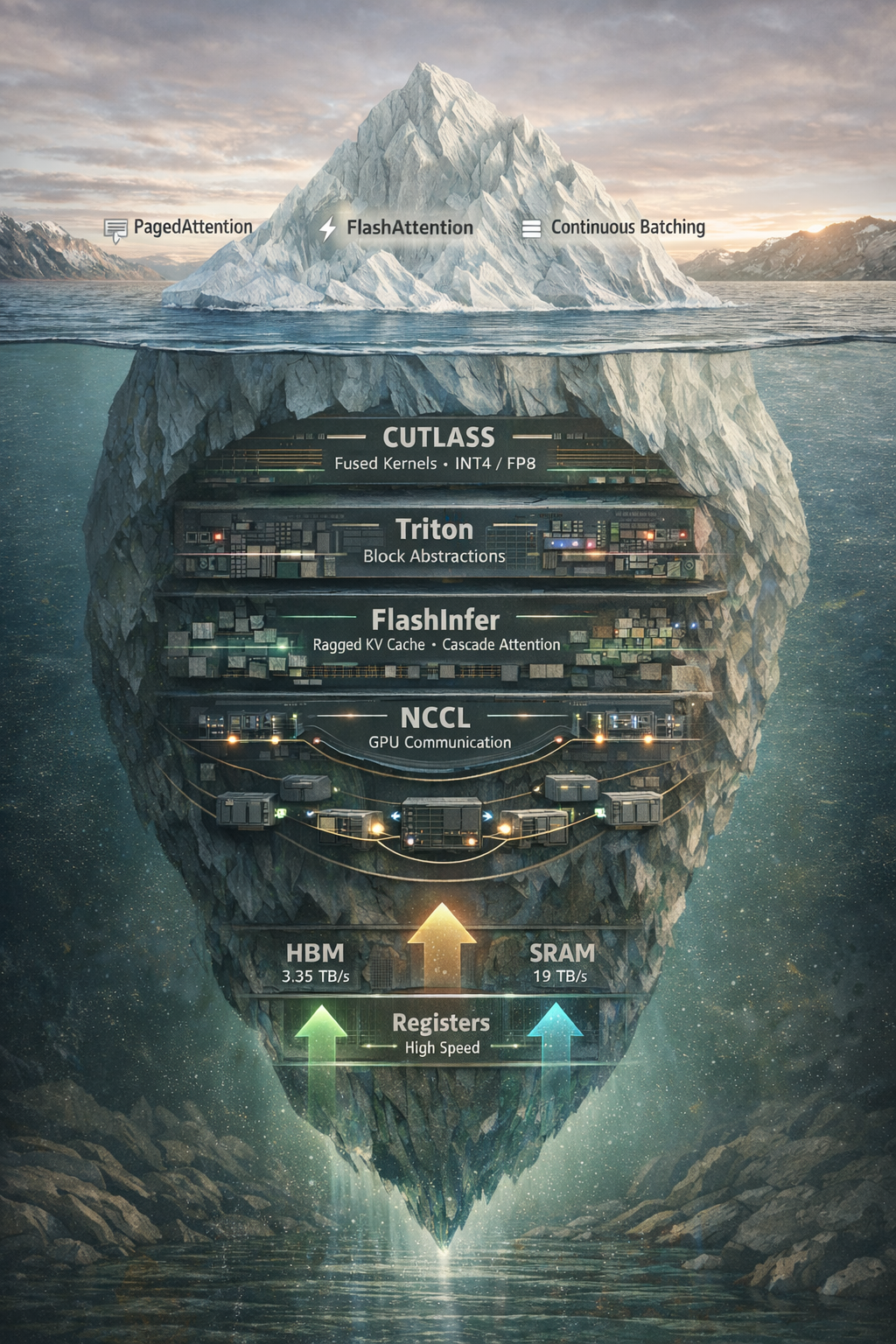
If you’ve followed LLM infrastructure over the past two years, you’ve probably heard the greatest hits: PagedAttention eliminates memory fragmentation, continuous batching keeps GPUs busy, and FlashAttention cuts memory from O(N²) to O(N). These optimizations are real and important. They are not the full story.
Below the waterline sits a stack of specialized libraries that most engineers never encounter directly. CUTLASS generates the fused kernels that make quantization practical. Triton lets researchers write GPU code without drowning in thread indexing. FlashInfer handles the messy reality of serving workloads that FlashAttention wasn’t designed for. And NCCL quietly orchestrates communication when models span multiple GPUs.
This post dives into that hidden layer. We’ll trace the path from silicon to scheduler, examining the libraries that transform NVIDIA’s hardware capabilities into the fast inference you actually experience. If you’re deploying LLMs at scale, or simply curious about what happens beneath vLLM’s Python API, this is the stack worth understanding.
Hardware Contract
Every optimization in this stack exists because of a single physical constraint: the memory wall. Modern GPUs have a dramatic imbalance between compute capability and memory bandwidth.
Consider the H100. Its Tensor Cores can deliver roughly 2,000 TFLOPS of FP8 compute. Its HBM3 memory provides 3.35 TB/s of bandwidth. Simple division gives us a “ridge point” of about 600 ops/byte—if your workload performs fewer than 600 operations per byte loaded from memory, you’re memory-bound. Your expensive Tensor Cores sit idle, waiting for data.
LLM inference during the decode phase operates at roughly 0.5-1 ops/byte. For every token generated, the model loads billions of weight parameters, multiplies them by a single vector, and discards the weights. It’s not even close to compute-bound. This is why a $30,000 GPU often achieves single-digit percentage utilization during autoregressive generation.
To understand why, it helps to see what we’re working with.
NVIDIA H100 GPU Architecture
Understanding the hardware that software must optimize for
Click components to explore
Streaming Multiprocessors
The memory hierarchy offers a path forward:
| Level | Capacity | Bandwidth |
|---|---|---|
| HBM (Global Memory) | 80 GB | 3.35 TB/s |
| L2 Cache | 50 MB | ~12 TB/s |
| SRAM (Shared Memory) | 228 KB/SM | ~19 TB/s |
| Register File | 256 KB/SM | Highest |
The software stack’s job is to maximize data reuse in faster memory levels and minimize trips to slow HBM.
GPU Memory Hierarchy: The Bandwidth Wall
Data flows through progressively faster, smaller caches to reach compute
The Memory Wall
CUTLASS: Template Metaprogramming Foundation
When you call a matrix multiplication in PyTorch, it eventually reaches cuBLAS—NVIDIA’s battle-tested linear algebra library. cuBLAS is fast, but it’s a black box. You get the GEMM you’re given.
For LLM inference, that’s often not enough. Consider what happens when you want to run an INT4 quantized model. The weights are stored as packed 4-bit integers. Before the Tensor Cores can process them, you need to:
- Load 128-bit vectors containing packed INT4 weights
- Unpack the 32-bit integers into eight 4-bit values
- Convert to FP16
- Apply quantization scales
- Feed the result to the Tensor Core
If each step is a separate kernel, you’re writing intermediate results to HBM between operations—exactly the memory traffic you’re trying to avoid. What you need is a single fused kernel that does everything in registers.
This is what CUTLASS enables. It’s NVIDIA’s header-only C++ template library for linear algebra, and it’s the foundation beneath vLLM’s quantization kernels, FlashAttention-3, and most high-performance transformer implementations.
When cuBLAS Won’t Cut It
Use CUTLASS when you need:
- Custom fusions: Bias + activation + quantization in one kernel
- Specific precision combinations: FP8 weights with FP16 accumulation
- Binary size constraints: cuBLAS ships megabytes of kernels for all cases
The trade-off is complexity. CUTLASS kernels require understanding GPU architecture at a level most ML engineers never encounter. But for the performance-critical paths in inference—attention, FFN, quantized projections—that complexity pays dividends.
Triton: GPU Programming Without the Pain
CUTLASS offers maximum control, but its learning curve is steep. Writing CUDA C++ means managing thread indices, avoiding bank conflicts, ensuring coalesced memory access, and reasoning about warp-level synchronization. A single misplaced __syncthreads() can introduce subtle bugs. A suboptimal memory access pattern can halve performance.
Triton takes a different approach. Developed by OpenAI and now integral to PyTorch 2.0, it raises the abstraction level from threads to blocks.
The Mental Model Shift
Traditional CUDA asks: “I am thread 47. What should I do?”
Triton asks: “I am processing this block of data. What operations should happen?”
Consider loading data from memory. In CUDA, you calculate addresses, handle boundary conditions, and coordinate across threads for coalescing. In Triton:
@triton.jit
def kernel(x_ptr, output_ptr, N, BLOCK_SIZE: tl.constexpr):
    pid = tl.program_id(0)
    offsets = pid * BLOCK_SIZE + tl.arange(0, BLOCK_SIZE)
    mask = offsets < N
    x = tl.load(x_ptr + offsets, mask=mask)
    # Process x...
    tl.store(output_ptr + offsets, result, mask=mask)
The tl.load call handles coalescing and vectorization automatically. The compiler figures out the optimal memory access pattern. No manual thread indexing or bank conflict avoidance.
The PyTorch Connection
When you call torch.compile() on a model, TorchInductor generates Triton kernels for GPU execution. The fusion engine identifies sequences of pointwise operations (add, multiply, activation) that can be combined into single kernels. Instead of three separate kernels with intermediate HBM writes, you get one kernel that loads data once, performs all operations in registers, and stores once.
A fused LayerNorm + Linear that would require 500+ lines of optimized CUDA takes about 50 lines of Triton. The resulting kernel won’t match a hand-tuned CUTLASS implementation, but it’ll be close, and it takes hours to write instead of weeks.
FlashInfer: Built for Serving
FlashAttention changed attention computation by recognizing that the bottleneck was memory I/O, not FLOPs. By computing attention tile-by-tile in SRAM and never materializing the N×N attention matrix in HBM, it reduced memory access from O(N²) to O(N). This brought longer context lengths and faster training.
But FlashAttention was designed for training workloads with regular, rectangular batches. Production serving is messier.
The Serving Reality
In a real serving deployment:
- Requests arrive with different context lengths (no neat rectangular batches)
- The KV cache uses PagedAttention with non-contiguous memory blocks
- Multiple requests share common prefixes (system prompts, document context)
- CUDA graphs need static shapes, but batch composition changes every iteration
FlashAttention handles none of this natively. FlashInfer does.
What FlashInfer Adds
Block-sparse KV cache support: FlashInfer kernels operate on PagedAttention’s block-sparse representation directly. Page tables map logical token indices to physical memory blocks, and FlashInfer traverses them efficiently without requiring contiguous memory.
Ragged tensor layouts: Standard kernels assume rectangular batches, padding shorter sequences to match the longest. FlashInfer operates on “ragged” layouts where sequences are packed tightly. No wasted compute on padding tokens.
Plan/run separation: FlashInfer separates scheduling decisions from kernel execution. The “plan” phase precomputes work distribution based on current batch composition. The “run” phase executes with that plan. This separation enables CUDA graph capture—record the run phase once, replay it with different inputs.
Cascade attention: When multiple requests share a common prefix (a system prompt, a retrieved document), naive approaches recompute attention over that prefix for every request. FlashInfer’s cascade attention processes the shared prefix once, caches the result, and computes only the unique suffix per request. For a 32K shared prefix across 256 requests, this yields a 31x speedup.
Integration with vLLM
vLLM’s attention backend isn’t monolithic. A kernel selection layer examines the workload (hardware architecture, head dimension, precision, model type) and dispatches to the appropriate backend: FlashAttention for standard cases, FlashInfer for PagedAttention scenarios, Triton for specific configurations. This flexibility means you get optimized kernels for your actual workload, not a one-size-fits-all solution.
NCCL: The Invisible Communication Backbone
Everything discussed so far assumes the model fits on a single GPU. For frontier models, it doesn’t. Llama-70B requires roughly 140GB in FP16—nearly two H100s worth of memory. Larger models require more.
Tensor parallelism splits the model across GPUs within a server. Weight matrices are sharded so each GPU holds a slice. Each GPU computes a partial result, and then… they have to talk to each other.
This is NCCL’s domain.
The Communication Pattern
Tensor parallelism using the Megatron-LM algorithm requires two AllReduce operations per transformer layer:
- After attention output projection: Each GPU computed attention over its head subset. AllReduce combines the results.
- After FFN down projection: Each GPU computed a partial FFN result. AllReduce sums them.
AllReduce means “sum tensors across all GPUs and distribute the result to all GPUs.” For Llama-70B on 4 GPUs, each AllReduce moves batch_size × sequence_length × hidden_dim × bytes_per_element bytes—and it happens 160 times per forward pass (2 per layer × 80 layers).
The Interconnect Gap
The choice of interconnect dominates multi-GPU inference performance:
| Interconnect | Bandwidth |
|---|---|
| NVLink 4.0 | 900 GB/s bidirectional |
| PCIe Gen5 | 128 GB/s bidirectional |
That’s a 7x gap. On NVLink, tensor parallelism adds modest overhead. On PCIe, communication becomes the bottleneck rather than memory bandwidth.
Even optimized, communication overhead consumes 20-35% of inference time for Llama-70B on 4×H100. It’s the reason single-GPU inference (when the model fits) is always preferable, and why quantization to fit larger models on fewer GPUs often improves overall throughput despite the precision loss.
Putting It Together
During decode, a single token flows through the entire stack: vLLM schedules the batch, PyTorch dispatches through CUDA graphs, and each transformer layer executes CUTLASS GEMMs for projections (with fused quantization), FlashInfer kernels for attention over the paged KV cache, and NCCL AllReduces if using tensor parallelism.
The time breakdown tells the story:
- Attention kernels: 40-60%
- FFN/MLP kernels: 30-40%
- Communication (with TP): 20-35%
- Everything else: <10%
Attention and FFN dominate. Both are memory-bound.
The Memory Bandwidth Endgame
Every library in this stack attacks the same fundamental constraint: memory bandwidth. CUTLASS enables fused kernels that minimize HBM round-trips. Triton makes writing such kernels accessible. FlashInfer optimizes attention’s memory access patterns. NCCL minimizes communication overhead that competes for the same memory bandwidth.
The hardware is evolving in the same direction. NVIDIA’s Blackwell B200 delivers 8 TB/s of HBM bandwidth, 2.4x more than H100, and introduces native FP4 support, halving bytes-per-parameter.
Understanding this stack is not just an academic exercise. If you’re deploying LLMs at scale, these libraries determine your cost per token, your latency percentiles, your maximum context length. The optimizations that matter aren’t in the model architecture; they’re in the software that maps that architecture onto silicon.
The iceberg runs deep. Now you know what’s beneath the surface.