Kimi K3's Architecture: Kimi Delta Attention, Attention Residuals, and 896 Experts

What this post covers

Moonshot AI published the Kimi K3 weights on 26 July 2026 and the technical report the following day. It is a mixture of experts with 2.78 trillion total parameters and 104.2 billion active per token, across 93 layers, with 896 routed experts and a one-million-token context window. The MXFP4 checkpoint comes to roughly 1.4 terabytes, so loading it takes a full node of accelerators.

Here is the idea the architecture turns on, stated up front. Letting every item on an axis see every other costs $O(n^2)$, so what that costs depends on how long the axis is. K3 moves information along three axes of very different lengths: the sequence is a million tokens, the width is 896 experts, and the depth is 93 layers grouped into 9. That difference is why K3 replaces softmax with a recurrence on three sequence layers in every four, and in the same model installs softmax attention on the depth axis where a plain residual connection used to be. Two moves in opposite directions, on two axes four orders of magnitude apart in length.

	Kimi K2	Kimi K3
Total parameters	1.04T	2.78T
Active per token	32.6B	104.2B
Layers	61	93
Attention	61 MLA	69 KDA + 24 Gated MLA
Positional encoding	RoPE	none (NoPE)
Routed experts / active	384 / 8	896 / 16
Shared experts	1	2
Hidden dim / MoE latent dim	7,168 / n/a	7,168 / 3,584
Activation	SwiGLU	SiTU-GLU
Training context	128K	1M

The attention design was validated first on Kimi Linear, a 48B model published in October 2025, where it cut KV-cache usage by up to 75% and delivered up to 6× the decoding throughput at a one-million-token context, with time per output token at 1M falling from 11.48 ms to 1.84 ms against full MLA. Those figures belong to the 48B model rather than to K3, which does not publish equivalents. On independent leaderboards K3 places fourth of 580 on Artificial Analysis’ index, second on Vals, and first on WebDev Arena, making it the first open-weights model to top that board.

Who this is for. Someone who knows how a Transformer works and has met attention and mixture-of-experts before, but has not read the K3 report. Where the argument leans on something specific I link out rather than re-explain it: multi-head latent attention, linear attention and the Mamba lineage, and rotary embeddings.

What this leaves out. There is nothing here on the vision tower, the Per-Head Muon optimiser, post-training, or what the design costs to serve, each of which would need its own post.

The three axes, and what softmax costs on each

Let’s start with the architecture as a whole. Moonshot’s overview figure lays it out along the same three axes:

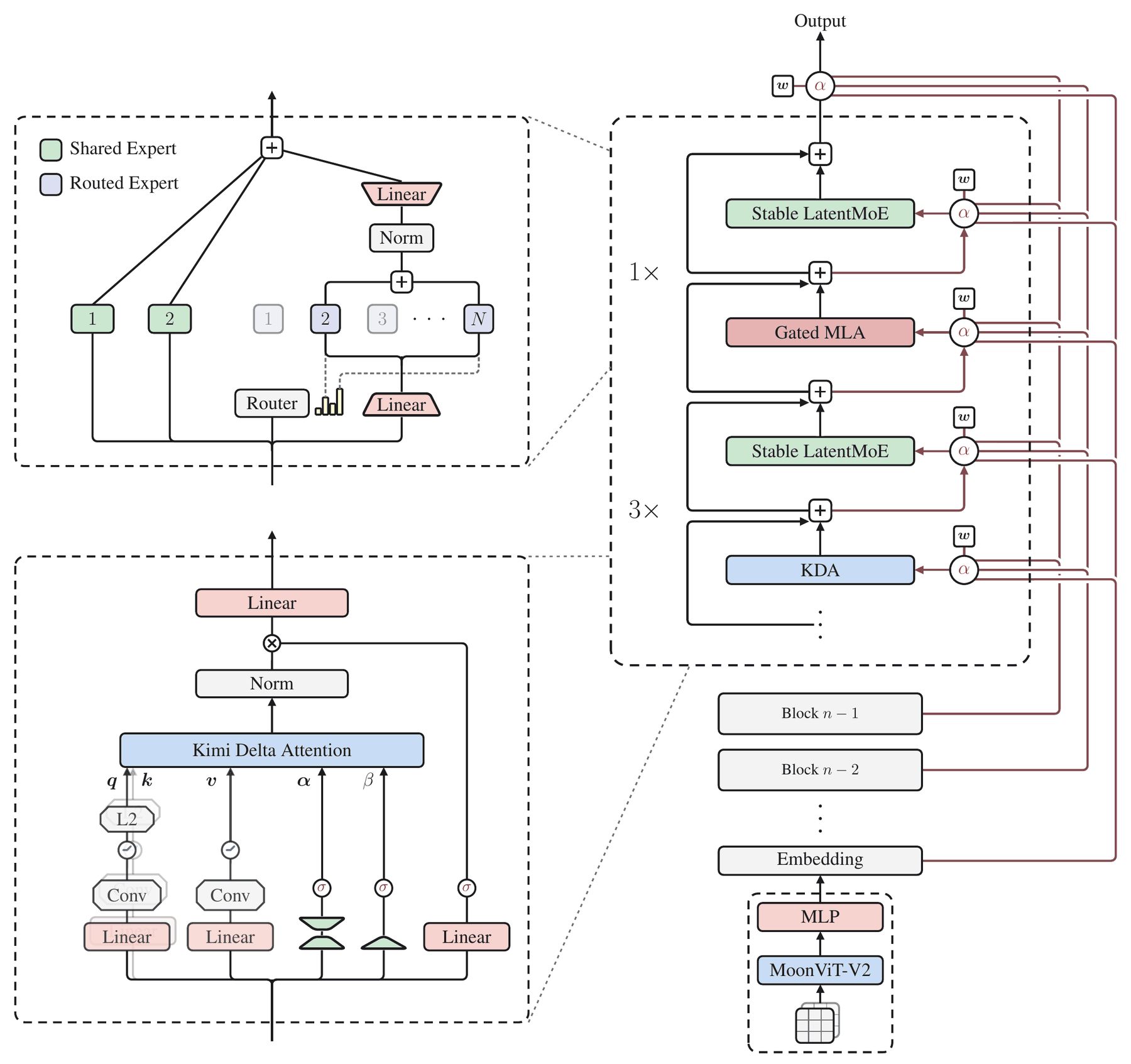
Figure 2 of the Kimi K3 technical report, reproduced without alteration. Kimi Team, Kimi K3: Open Frontier Intelligence.

Reading the right-hand column from the bottom, the 3:1 ratio is visible directly: KDA, then a LatentMoE, three times over, then one Gated MLA and a final LatentMoE to close the block. The two boxed insets on the left are the modules we spend most of our time inside. The maroon lines fanning from every module back down to Block n-1, Block n-2 and Embedding are Attention Residuals, which is the depth axis drawn as wiring.

A million tokens, 896 experts, and 93 layers grouped into 9 are three very different lengths, and they set very different prices. The sequence axis carries much the largest, since at a million tokens a single head in a single layer scores $n^2 = 10^{12}$ query-key pairs, and causal masking only halves that. Expensive as this is, it stops well short of impossible, and K3 pays it on the 24 layers where it keeps full attention. What binds is not the prefill but the decode that follows it, because every generated token has to read the whole KV cache before it can produce the next one, so time per output token climbs with context rather than holding flat.

Depth asks the same question of a far smaller number. K3 has 93 layers, and because Block AttnRes groups them into 9 sources the operative $n^2$ is 81 rather than 8,649. Neither figure is large enough to trouble anything, and the report is blunt about it:

Since network depth is modest ($L \lt 100$), the $O(L^2 d)$ arithmetic of this full form is affordable.

Width is where the accounting changes character rather than scale. There are 896 experts in a layer, but no expert ever attends over another: the router scores each one on its own, so the work grows linearly with the expert count and no pairwise term arises to be paid at all. What constrains the axis instead is that every expert selected costs a matrix multiply, which is why a model can afford $k$ of them and not $n$. Routing densely to all 896 would cost $E/k = 56$ times what top-$k$ costs, and a factor of 56 is a linear penalty where the sequence axis faced a quadratic one. Width stays hard top-$k$ for that reason, and the problems that make it interesting turn out to lie elsewhere.

Let’s put the three side by side:

Softmax is affordable where the axis is short, and depth is much the shortest. Depth has not gone unexamined: Highway Networks put learned gates on the residual in 2015, DenseNet wired every layer to every later one in 2016, and DeepSeek-V4 ships manifold-constrained hyper-connections to the same end. What those share is that the mixing is fixed or input-gated. What AttnRes changes is the weighting, from a constant to a content-dependent softmax, which is the move the sequence axis made in 2017 and the width axis has never made at all.

The sequence axis: linear attention and a fixed-size state

Let’s start with what has to go. The quadratic score matrix is the part people name first, and it is also the part that is already solved: FlashAttention computes exact attention without ever materialising the $n \times n$ matrix. What has no fix of that kind is the KV cache. It is linear in context, so decoding a single token means streaming the entire history out of memory, and that happens again for every token generated. Multi-head latent attention shrinks the per-token cost of that cache by a large constant factor, and a large constant factor is not enough when the thing it multiplies is $10^6$.

Linear attention takes the other road. Instead of keeping every past token and searching them at read time, keep a fixed-size summary and update it as you go. The state is a matrix $S_t \in \mathbb{R}^{d_k \times d_v}$, written with outer products and read with a matrix-vector product:

$$S_t = S_{t-1} + k_t v_t^\top, \qquad o_t = S_t^\top q_t$$

This is an associative memory. Writing the pair $(k_t, v_t)$ adds a rank-one term. Reading with a query $q$ that happens to equal some stored $k_i$ returns $v_i$ plus whatever the other stored pairs contribute along that direction. The cost per token no longer depends on how many tokens came before, because there is only ever one $S$.

That saving has a cost, and it arrives immediately. $S$ has $d_k \times d_v$ entries and that number never grows, so past a certain point new information can only be stored by degrading what is already there. In K3, $d_k = d_v = 128$, which gives each head 16,384 numbers to work with and nothing more.

Before we pay for that, here is what it buys. K3 keeps 24 Gated MLA layers out of 93, and only those layers hold a cache that grows with context; the other 69 hold a fixed-size state instead:

That is the constraint the rest of this axis has to work around. Anything written early has to survive most of a million subsequent writes into the same fixed state, and every one of those writes is a chance to corrupt it.

Deriving the delta rule

The update above has an obvious failure mode. Suppose the sequence writes $(k, v_1)$ early and $(k, v_2)$ later, with the same key. The state now holds $k v_1^\top + k v_2^\top$, and reading with $q = k$ returns a blend of both values weighted by $\lVert k \rVert^2$. The memory did not update the association, it superposed two of them. Do this a few thousand times and reads return an average of everything ever written to nearby keys.

The fix is to treat the write as an optimisation step rather than an addition, and ask the memory to reduce its own retrieval error. We define the loss as the squared distance between what the memory currently returns for $k_t$ and what it should return:

$$\mathcal{L}_t(S) = \tfrac{1}{2}\big\lVert S^\top k_t - v_t \big\rVert^2, \qquad \nabla_S \mathcal{L}_t = k_t\,\big(S^\top k_t - v_t\big)^\top$$

Now we take exactly one gradient step from $S_{t-1}$, with step size $\beta_t$:

$$S_t = S_{t-1} - \beta_t\, k_t \big(S_{t-1}^\top k_t - v_t\big)^\top$$

Expanding the bracket and collecting the terms that involve $S_{t-1}$:

$$\boxed{\;S_t = \big(I - \beta_t k_t k_t^\top\big)\,S_{t-1} + \beta_t k_t v_t^\top\;}$$

That is the delta rule, and it came out of asking a linear associative memory to perform one step of gradient descent on its own reconstruction error. Nothing else went into it. The $\beta_t k_t v_t^\top$ term is the write we already had; the new factor $\big(I - \beta_t k_t k_t^\top\big)$ is the correction. Since KDA normalises its keys, $\lVert k_t \rVert = 1$, and $I - k_t k_t^\top$ is then the orthogonal projector that removes the $k_t$ component of whatever it multiplies. So at $\beta_t = 1$ the update erases whatever the memory currently associates with $k_t$ and writes $v_t$ into the space it cleared. At $\beta_t \lt 1$ the erasure is partial, which is why the report calls $\beta_t$ the write strength.

Below we can write a few pairs into the memory, reusing keys, and see what the projector does:

What the projector guarantees can be read straight off the update. We want to know what the memory returns for the key just written, so we set $q = k_t$:

$$o_t = S_t^\top k_t = \underbrace{(1-\beta_t)\,S_{t-1}^\top k_t}_{\text{what survived the erasure}} + \;\beta_t v_t$$

At $\beta_t = 1$ the first term vanishes and the read returns $v_t$ exactly, which is why the newest key in the panel sits at error 0.000 however crowded the state already was. The most recent write is exact, and that is all the rule promises.

Older keys drift. Every subsequent write erases along a direction close to, but not quite, orthogonal to theirs, so their values degrade a little each time. With the projector switched off both problems appear at once: even the newest key comes back wrong, and mean error runs about three times higher.

The delta rule governs what happens to a key when we write to it and says nothing about the keys we stop writing to, which at a million tokens is most of them.

Channel-wise decay, and the floor K3 puts under it

So we add decay. Multiply the state by a retention factor before each write, and old content fades unless it is refreshed. KDA’s full recurrence is the delta rule with exactly that inserted:

$$S_t = \big(I - \beta_t k_t k_t^\top\big)\,\underbrace{\mathrm{Diag}(\alpha_t)}_{\text{channel-wise decay}}\,S_{t-1} + \beta_t k_t v_t^\top, \qquad \tilde{o}_t = S_t^\top q_t$$

The detail that matters is that $\alpha_t \in (0,1)^{d_k}$ is a vector, not a scalar. Mamba-2 and Gated DeltaNet, both of which this line descends from, use one decay value per head. KDA gives every one of the 128 key channels its own retention rate, computed per token from a low-rank projection of the hidden state plus a per-head bias.

Suppose some fact has to stay legible across a million tokens. The channel carrying it needs a per-step retention $\alpha$ with $\alpha^{N}$ still meaningfully above zero at $N = 10^6$; setting $\alpha^{N} = \tfrac{1}{2}$ and solving gives $\alpha = 2^{-10^{-6}}$, which sits less than one part in a million below 1. Meanwhile the same head is tracking things like bracket depth, the current scope, and which file it is reading, all of which should be flushed within a few tokens. A single scalar per head has to satisfy both demands with one number, and it cannot. A diagonal lets channel 47 sit at $1 - 10^{-6}$ while channel 12 sits at $0.01$ and clears itself twice a line.

The next change is what separates K3 from Kimi Linear. It concerns how the decay is parameterised, and the justification for it has nothing to do with modelling.

Chunkwise linear attention processes the sequence in chunks, parallel inside a chunk and recurrent across chunks. Inside a chunk we need the decay from each position to every later position, and the standard way to get it is to compute the cumulative decay $\Gamma^{1 \to C}$ once and divide. Concretely, from the report’s Eq. 4, the intra-chunk term rescales keys by the reciprocal $1/\Gamma^{1\to C}$. That reciprocal is one over a product of numbers smaller than 1, and it grows without bound.

Kimi Linear used an unbounded log-decay, $g = -e^{A}\,\mathrm{softplus}(z)$, which lives in $(-\infty, 0)$. Under that parameterisation the reciprocal really can overflow, so Kimi Linear split each chunk into 16-token secondary tiles and computed the off-diagonal tiles as dense matrix multiplications while the diagonal tiles fell back to explicit position-pair arithmetic. The report names that fallback as the main intra-chunk bottleneck.

K3 changes the mapping to a scaled sigmoid with a floor:

$$g_t = g_{\min}\cdot\sigma\!\left(e^{A_h} z_t\right) \in (g_{\min},\, 0), \qquad \alpha_t = \exp(g_t) \in \left(e^{g_{\min}},\, 1\right), \qquad g_{\min} = -5$$

Let’s follow the arithmetic through. With $g_{\min} = -5$, every retention factor exceeds $e^{-5} \approx 6.7 \times 10^{-3}$. Cumulative log-decay across a 16-token tile therefore lies in $(-80, 0)$, so the reciprocal rescaling factor is bounded by $e^{80} \approx 5.5 \times 10^{34}$. BF16 tops out around $3.4 \times 10^{38}$. It fits, with about four orders of magnitude to spare, and it fits by construction. Every causal tile, diagonal included, then becomes a dense Tensor Core matmul, and the position-pair path is removed from the kernel entirely.

Dragging the floor moves both consequences together:

Let’s be precise about what this trade costs. A floor on the log-decay bounds how fast a channel may forget. It places no ceiling on how long a channel may remember, since the upper end of $\alpha$ is still an open interval approaching 1, so a channel holding a long-range fact is unaffected. What the bound removes is the ability to zero a channel in a single step, and a channel sitting at $\alpha = 6.7\times10^{-3}$ still discards 99.3% of its content per token, which clears local state about as fast as anything would need.

This pattern shows up repeatedly in the K3 report: the mathematics is constrained so that the kernel can get simpler, and the constraint is placed where the model was not using the range anyway. The architecture is being shaped to fit the hardware rather than the other way round.

NoPE: position from the recurrence

K3 applies no positional encoding at all to its 24 Gated MLA layers. No rotary embeddings, no ALiBi, nothing. Queries and keys go into global attention carrying only content.

That works because the KDA layers already encode position, and they do it structurally rather than by addition. A recurrence with a learned per-channel decay is inherently order-sensitive: the state at token $t$ depends on the sequence of decays applied since each earlier write, so $\alpha^{t-i}$ acts as a learned, data-dependent, multiplicative analogue of the fixed sinusoidal factors in rotary embeddings. Position falls out of the dynamics instead of being injected into the representation. With three KDA layers before every MLA layer, by the time a token reaches global attention its representation is already positioned.

The payoff shows up in the long-context curriculum. The report extends the window in four stages, 8K to 64K during pre-training and 256K to 1M during cooldown, and it says the model “extrapolates directly to 1M-token contexts without any positional-encoding modification, such as RoPE rescaling or interpolation.” Every long-context model since 2023 has fought a version of this fight: your rotary base was fitted at one length, you want to serve at another, so you stretch the frequencies uniformly or unevenly and hope the model tolerates the surgery. K3 has nothing to stretch. Removing the positional encoding removed the thing that needed retuning.

As far as I can tell this is the strongest novelty claim available for K3: it is the first frontier-scale model to run NoPE across every layer rather than in a subset of them.

The depth axis: what a residual connection computes

Now the other direction. In a standard residual network each layer adds its own output to the stream it received:

$$h_l = h_{l-1} + f_{l-1}(h_{l-1})$$

Substituting the same rule for $h_{l-1}$ gives

$$h_l = \underbrace{h_{l-2} + f_{l-2}(h_{l-2})}_{h_{l-1}} + f_{l-1}(h_{l-1})$$

and doing it again for $h_{l-2}$, and again below that, peels off one term at a time while leaving everything already peeled untouched. Carried down to the embedding, the recursion telescopes into a plain sum:

$$h_l = h_0 + \sum_{i \lt l} f_i(h_i)$$

Each $f_i$ is still evaluated at its own input $h_i$ rather than at $h_0$, so this is an accounting identity rather than a closed form in the embedding. It tells us what the stream at layer $l$ is made of, which is the part we need.

Read that sum as an aggregation. Every earlier layer’s output arrives with weight exactly 1, and that weight is not learned, does not depend on content, and is not normalised. Uniform aggregation with constant coefficients is what attention reduces to when the scores are constant and the softmax is removed, so a residual stream has been doing depth-wise linear attention since 2015. It is not usually described that way, though the family is a familiar one. Highway gates and DenseNet wiring are both weightings over depth, and what they share with a plain residual is that the weight does not depend on what the layer said.

Two things go wrong as $L$ grows, and the AttnRes paper names both. First, dilution: in a 93-layer sum, any individual layer’s contribution is about 1.1% of the stream, so early information is progressively drowned by everything written after it. Second, uncontrolled growth: the sum is unnormalised, so the magnitude of $h_l$ grows with depth, and later layers have to emit ever-larger outputs to move the stream at all.

Neither of those is a cost problem. Attending over depth was affordable in 2015 and is free now. What was missing was a reason to want it, and dilution across 93 layers is that reason.

We can compare the two aggregations directly by toggling between uniform weights and learned ones:

The magnitude trace on the right is the one to look at, because it explains why the two problems have a single fix. Uniform accumulation is an unbounded sum, so the stream grows monotonically with depth and each layer’s relative influence shrinks whether or not it had anything useful to contribute. A softmax produces a convex combination instead: weights that are non-negative and sum to 1, which bounds the result by the largest term being combined. Normalising the weights is what fixes the dilution, and it is also what stops the growth.

To make that concrete: a token’s embedding enters the stream at layer 0, and some computation near the top of the stack may still need it. Under uniform accumulation, layer 88 receives that embedding as roughly one percent of a stream into which 87 other layers have also written. What we want is for layer 88 to be able to ask for it.

Attention Residuals: one learned query per layer

The mechanism is small. We give each layer $l$ a single learnable pseudo-query $w_l \in \mathbb{R}^d$, and let the keys and values be the outputs of all preceding layers, with the token embedding at index 0 so that it is always available as a source:

$$k_i = v_i = \begin{cases} h_1 & i = 0 \\ f_i(h_i) & 1 \le i \le l-1\end{cases}$$

We score with an exponential kernel over RMS-normalised keys, then normalise across depth:

$$\alpha_{i\to l} = \frac{\exp\!\big(w_l^\top\, \mathrm{RMSNorm}(k_i)\big)}{\sum_{j \lt l}\exp\!\big(w_l^\top\, \mathrm{RMSNorm}(k_j)\big)}, \qquad h_l = \sum_{i \lt l} \alpha_{i\to l}\, v_i$$

Three choices here are doing real work. The RMSNorm on keys exists because unnormalised residual streams grow with depth, so without it a late layer would win the attention on magnitude alone rather than on content. The softmax, rather than a sigmoid, makes the weights competitive: a layer that attends more to the embedding necessarily attends less to something else, which is what forces it to choose. And the query is one vector per layer rather than one per token, so what gets learned is a position-independent preference over depth. That is also why it costs so little.

There is no per-token routing over depth, and the ablations in the AttnRes paper find that multi-head depth attention makes results worse rather than better.

The practical problem is memory. Full AttnRes needs every preceding layer’s output kept alive, which is $O(Ld)$ memory and, under pipeline parallelism, $O(Ld)$ cross-stage communication. The arithmetic was affordable; the memory traffic is not. Block AttnRes is the fix: K3 groups its 93 layers into 8 blocks of 12, sums ordinarily inside a block, and attends only over the block-level summaries. Counting the embedding, that leaves 9 sources rather than 93, and the memory that has to be kept alive falls by an order of magnitude with it.

A late layer can then put real weight on the block holding what it needs, rather than receiving it as one percent of an undifferentiated sum.

The width axis: 896 experts and the cost of dispatch

Sparsity on this axis, the ratio of pool to active, rises from K2’s 48 to K3’s 56, and the obstacle to raising it is traffic rather than parameter count. In a conventional mixture of experts, each selected expert receives the full $d$-dimensional token representation, so doubling the number of active experts doubles both the all-to-all communication and the expert weight traffic. At $d = 7168$ and 16 active experts, that communication cost is the binding constraint.

LatentMoE separates the model’s width from the routed experts’ width. Shared experts keep the full-width path, while routed experts work in a compact latent space of width $\ell$, reached by a down-projection before dispatch and mapped back afterwards:

$$u = \sum_{i \in T_k(x)} p_i\, E_i^{\text{routed}}(W_{\downarrow} x), \qquad y = \sum_{j} E_j^{\text{shared}}(x) + W_{\uparrow}\,\mathrm{RMSNorm}(u)$$

K3 sets $\ell = 3584$, exactly half the hidden dimension, so the tokens crossing the network for dispatch are half-width. The arithmetic works out exactly: K2 moved $8 \times 7168 = 57{,}344$ values per token, and K3 moves $16 \times 3584 = 57{,}344$. Twice the routing multiplicity for an identical communication bill, which is what makes 16-of-896 affordable at all.

Sparsity at that level amplifies two failure modes already present in the vanilla design, and the report is unusually direct about both. The routed path runs through $W_{\downarrow}$, then a gated multi-branch expert network, then $W_{\uparrow}$, which the report calls “a chain of nearly four consecutive matrix multiplications”; that ill-conditioned structure at 2.8 trillion parameters produces exploding activations in the routed branch. Balancing the load of nearly $10^3$ experts, meanwhile, “exceeds the regime in which existing auxiliary-loss-free bias updates remain well behaved.”

Bounding the activations

The activation problem gets the smaller fix. SwiGLU multiplies two unbounded factors, so coincident large coordinates produce activation outliers, and outliers are exactly what low-precision arithmetic handles worst. The original GLU’s sigmoid gate is bounded but loses the roughly linear positive response that makes Swish work.

SiTU-GLU applies a smooth cap, $\mathrm{softcap}(x,\beta) = \beta\tanh(x/\beta)$, to the linear factor of the Swish gate and independently to the up branch:

$$\text{SiTU-GLU}(x) = \beta_1\tanh\!\left(\frac{W_g x}{\beta_1}\right) \odot \sigma(W_g x) \odot \beta_2\tanh\!\left(\frac{W_u x}{\beta_2}\right)$$

K3 uses $\beta_1 = 4$ for the gate branch and $\beta_2 = 25$ for the up branch. Three properties follow from that, all worked in Appendix B. Near the origin $\beta\tanh(z/\beta) = z + O(z^3/\beta^2)$, so SiTU-GLU matches SwiGLU to first order where most activations live. As $\beta_1,\beta_2 \to \infty$ it recovers SwiGLU pointwise, so the design is a strict generalisation. And since $\lvert\tanh\rvert \lt 1$ and $0 \lt \sigma \lt 1$, every output coordinate obeys

$$\lVert \text{SiTU-GLU}(x)\rVert_\infty \le \beta_1\beta_2 = 100$$

A hard clamp would bound the output too, and the report explains why it was not used: the smooth cap keeps gradients nonzero away from the saturation boundary, whereas a clamp sets them to exactly zero and the unit stops learning.

That leaves the balancing problem, which needs more than a bound.

Quantile balancing

Mixture-of-experts models need their experts used evenly. An expert that receives too few tokens trains poorly and eventually dies; an expert that receives too many becomes a straggler that every other device waits on.

Some notation first, since the rest of this section leans on it. Take a batch of $m$ tokens and $n$ experts, with every token routed to $k$ of them; in K3, $n = 896$ and $k = 16$. The router emits a score $s_{i,j}$ for each token $i$ and expert $j$, and we write $s_{:,j}$ for the whole column of scores belonging to expert $j$, one per token in the batch. Let $c_j$ be that expert’s load, meaning the number of tokens actually routed to it, and $\bar{c}$ the average load across experts. Perfect balance would put every expert at the target load

$$q = \frac{mk}{n}$$

since the batch hands out $mk$ routing slots in total and there are $n$ experts to share them.

The modern approach, from DeepSeek-V3, avoids auxiliary losses and instead maintains a per-expert bias $b_j$ that is added to the router score for top-$k$ selection and omitted from the mixture weights, so it steers dispatch without touching gradients. After each step $t$, every bias moves one fixed increment $\gamma$ in the direction of its own load error:

$$b_j^{(t+1)} = b_j^{(t)} + \gamma\,\mathrm{sign}\big(\bar{c} - c_j\big)$$

An expert sitting below the average has its bias raised, which makes it win more top-$k$ contests on the next step; one sitting above the average has its bias lowered.

At 384 experts $\gamma$ can be tuned. At 896 there is no good value for it: a small $\gamma$ takes too many steps to equilibrate, and during those steps some experts are receiving almost nothing to train on, while a large $\gamma$ overshoots and the loads oscillate. The underlying reason is that the update carries only the direction of the load error and discards its magnitude, so the step size is being asked to guess how far to move.

Quantile Balancing removes the step entirely. Route with top-$(k{+}1)$ rather than top-$k$: the first $k$ entries are the routes actually taken, and the $(k{+}1)$-th biased score is the cutoff $\alpha_i$ that an expert has to beat to enter token $i$’s selection. Holding those cutoffs fixed, expert $j$ receives exactly the tokens whose margin $s_{i,j} - \alpha_i$ clears $-b_j$, so its load falls monotonically as $b_j$ falls. That makes the target load something we can solve for rather than approach. We want the bias at which exactly $q$ of the $m$ margins still clear it, and since $q/m = k/n$ that cut sits at the $(1-k/n)$-quantile of the margins:

$$\hat{b}_j^{(t+1)} \leftarrow -\,\mathrm{quantile}_{1-k/n}\big(s_{:,j} - \alpha^{(t)}\big), \qquad b^{(t+1)} \leftarrow \hat{b}^{(t+1)} - \mathrm{mean}\big(\hat{b}^{(t+1)}\big)$$

The hat marks the raw solution before centring. Subtracting the mean from every entry removes an offset shared by all experts, which cannot change a top-$k$ ranking and so costs nothing. The update applies at the next step, so a batch is never routed with a bias derived from itself, and the bias is frozen at inference.

The two rules are not rivals so much as two ways at the same problem. Appendix C of the report sets up the maximum-score balanced assignment, the routing that maximises total router score while giving every expert exactly $q$ tokens, and shows that its dual has a closed-form solution: precisely the quantile above. Quantile Balancing jumps straight to it.

DeepSeek’s rule turns out to be descending that same objective, one sign at a time. Its update is what you get by taking the gradient and keeping only its direction, and the gradient itself is $q - c_j$, the target load minus the observed one. The heuristic everyone shipped was already gradient descent on a problem that has an exact answer. That is why one of them needs a step size and the other does not, and why, in the report’s phrasing, Quantile Balancing “equilibrates within a few update steps even for nearly $10^3$ experts.”

Below we can run both rules on the same imbalanced routing and look for a step size that wins:

One engineering detail makes this practical at scale. The quantile is over the whole global batch, whose margins number in the millions and are sharded across ranks and accumulation steps, so gathering them exactly is not viable. K3 estimates each expert’s quantile from a histogram of its margins: bin locally, then a single all-reduce sums the per-rank bin counts. Because counts are additive, the pooled histogram represents the true global batch no matter how tokens were sharded, so the estimate is the whole-batch quantile up to the bin width, at a communication cost of a few hundred bins per expert. The approximation costs resolution rather than correctness: the statistic being computed is still the global one.

Where to get it

K3 is an open-weights release, so most of what is described above can be inspected directly.

• Weights: huggingface.co/moonshotai/Kimi-K3, MXFP4, roughly 1.4 TB.
• KDA kernels: FlashKDA is a CUTLASS implementation of the chunkwise algorithm used in the sequence-axis sections above, auto-dispatched as a backend of flash-linear-attention.
• Expert parallelism: MoonEP, the balanced all-to-all layer the width axis depends on during training.
• The 48B precedent: Kimi Linear, where this attention design was validated and where the KV-cache and throughput measurements quoted earlier come from.

What the report does not say

Two things to keep in mind before treating any of the numbers above as settled.

The training scale is not disclosed. Across 47 pages there is no pre-training token count, no total FLOPs, no GPU type or count, no cluster size, no MFU, no wall-clock, and no cost. The only hardware-scale figure in the paper is “within a few hundred GPUs”, and that refers to one co-located million-token RL experiment rather than to pre-training. Any article quoting a K3 training cost is quoting someone’s guess.

The headline 2.5× is an extrapolation from curves fitted far below the scale K3 was actually trained at. It is a scaling-efficiency ratio taken from fitted scaling-law curves for K2 and K3, and the x-axis of that figure spans only $10^{20}$ to $10^{21}$ FLOPs, while a 2.8-trillion-parameter production run sits orders of magnitude to the right of the plotted range. The report is straightforward about this and presents the number as an extrapolation from a hyperparameter sweep.

There is also a fair critique of the novelty. Sebastian Raschka’s read is that K3 is largely the Kimi Linear architecture scaled 58×, that LatentMoE closely resembles the design in Nemotron 3 Ultra and so is convergent rather than proprietary, and that AttnRes is the one component change that is not an efficiency tweak. I think that assessment is broadly right. The engineering that matters in K3 is less the invention of the parts than the discovery of what breaks when a validated 48B design is taken to 2.8T, together with the specific repairs.

What I take from this

Pulling the three axes back together: on the sequence axis K3 replaces softmax with a gated delta rule over a fixed-size state on three layers in four, with a decay floor chosen so the chunkwise kernel stays inside BF16. On the depth axis it does the opposite, replacing the plain residual sum with a softmax over nine block-level sources. On the width axis it keeps hard top-$k$ and repairs the balancing rule instead, by solving the dual that the old rule had been descending.

Reading the report through, what stayed with me is how much of K3 is repair work rather than invention. Two of the three axes arrived largely finished: Kimi Linear had validated the hybrid attention at 48B, and Attention Residuals had been validated at the same size in its own paper. Much of what is genuinely new at 2.8T answers a specific breakage instead. SiTU-GLU is there because a chain of four matmuls in the routed path made activations explode. Quantile balancing is there because the sign rule stops behaving somewhere between 384 and 896 experts. Even the decay floor, which reads like a modelling decision, exists to delete a slow path from the kernel rather than to fix anything the model was doing. None of that is glamorous, and all of it was necessary. That is probably the honest shape of most frontier engineering.

The depth axis is the part I keep coming back to. Attending over 9 block-level sources costs 81 pairwise scores per token, which was affordable on 2015 hardware and is free now. Depth has never been short of mixing schemes either, from Highway gates through DenseNet to hyper-connections. What took a decade was making the weighting depend on content, and cost was never what stood in the way. I keep turning that over, because it suggests the more useful question is less often what we cannot afford than which constants we never thought to make learnable.

There is a larger thing here than any of the three axes. K3 sits fourth of 580 on Artificial Analysis’ index and first of 99 on WebDev Arena, the first open-weights model to lead that board, and Moonshot published the weights, the kernels, the expert-parallel layer, and 47 pages of method alongside them. Every derivation in this post exists because that report exists. None of it needed access, a partnership, or a guess.

That is also why the post covers so little of the model. Three sections out of 47 pages leaves out the vision tower trained from scratch, Per-Head Muon, quantisation-aware training carried through reinforcement learning, a balanced expert-parallel layer with an existence proof attached, and the 51 million sandboxes the RL environments consumed. I set out to explain Kimi K3 and got as far as the attention, the residuals, and the router. The rest is sitting there, readable, which is not something I could have written about a frontier model two years ago.

References

1. Kimi Team (2026). Kimi K3: Open Frontier Intelligence. arXiv:2607.24653. The primary source for this post. Architecture in §2, pre-training in §3, infrastructure in §5, and the Quantile Balancing derivation in Appendix C.
2. Kimi Team (2025). Kimi Linear: An Expressive, Efficient Attention Architecture. arXiv:2510.26692. The 48B model K3’s hybrid attention was validated on. Source for the chunkwise KDA form and the 3:1 layer ratio.
3. Kimi Team (2026). Attention Residuals. arXiv:2603.15031. The AttnRes paper. Source for the dilution and unbounded-growth argument, the Block AttnRes construction, and the ablations on RMSNorm, softmax, and multi-head depth attention.
4. Kimi Team (2025). Kimi K2: Open Agentic Intelligence. arXiv:2507.20534. The predecessor. Source for the K2 column of the architecture comparison and for the weight-clipping mechanism K3 retains.
5. Elango, V. et al. (2026). LatentMoE: Toward Optimal Accuracy per FLOP and Parameter in Mixture of Experts. arXiv:2601.18089. The latent-routing design K3 builds Stable LatentMoE on.
6. Yang, S., Kautz, J., & Hatamizadeh, A. (2025). Gated Delta Networks: Improving Mamba2 with Delta Rule. ICLR 2025. The direct ancestor of KDA, and the source of the scalar-per-head decay that channel-wise gating replaces.
7. Schlag, I., Irie, K., & Schmidhuber, J. (2021). Linear Transformers Are Secretly Fast Weight Programmers. ICML 2021. The delta rule as an update to a linear associative memory.
8. Dao, T., & Gu, A. (2024). Transformers are SSMs: Generalized Models and Efficient Algorithms Through Structured State Space Duality. ICML 2024. Mamba-2, and the chunkwise parallel form that KDA’s algorithm follows.
9. DeepSeek-AI (2024). DeepSeek-V2: A Strong, Economical, and Efficient Mixture-of-Experts Language Model. arXiv:2405.04434. Multi-head latent attention, which K3 retains in its global layers.
10. Wang, L. et al. (2024). Auxiliary-Loss-Free Load Balancing Strategy for Mixture-of-Experts. arXiv:2408.15664. The origin of the fixed-step sign rule. K3’s report cites it as deployed in the DeepSeek-V3 Technical Report, which is the form Appendix C shows to be SignSGD on the same dual.
11. Lewis, M. et al. (2021). BASE Layers: Simplifying Training of Large, Sparse Models. ICML 2021. The assignment-problem view of expert load balancing that Appendix C traces its lineage to.
12. Dao, T. et al. (2022). FlashAttention: Fast and Memory-Efficient Exact Attention with IO-Awareness. NeurIPS 2022. Online softmax, which Block AttnRes reuses to merge inter-block and intra-block results.
13. Shazeer, N. (2020). GLU Variants Improve Transformer. arXiv:2002.05202. SwiGLU, and the unbounded product that SiTU-GLU caps.
14. Jordan, K. et al. (2024). Muon: An optimizer for hidden layers in neural networks. The optimiser K3 refines into its per-head variant.
15. Raschka, S. (2026). Kimi K3 Architecture Notes. The most useful sceptical read: K3 as Kimi Linear scaled 58×, LatentMoE as convergent with Nemotron 3 Ultra, and AttnRes as the one non-tweak.
16. Willison, S. (2026). Kimi K3. Hands-on notes and the pricing jump from K2.6.
17. Lambert, N. (2026). Open models recap: more on Kimi K3. On where the open-to-closed gap is narrow and where it is not.